1

I plot a second-order polynomial using the following code in Matlab:

 xx = 1 : 4000;
 mu =    1.0e+03 * [ 2.0733; 0.6569];
 b = 198;   
 P = [2.5577,   -1.0134,  102.4344];

 figure;imshow(img,'border','tight');
            hold on;
 plot(xx,polyval(P,xx,[],mu)+b,'LineWidth',1.5,'Color','r');

It results the following image:

enter image description here

However, if I comment out the figure;imshow(img,'border','tight'); it shows the following curve:

enter image description here

First, I don't know why these two plots differ and which is the right plot of the polynomial.

Second, I look for a measure for the degree of bending for the object shown in Figure 1, so that I be able to compare two objects with low or high bending (curvature). However, I don't know how to extract such a measure from the polynomial formula. I tried to use the coefficient of x^2 (P(2)), but I am not sure if it is a representative of the curve in Figure 1, because Figure 2 shows something different.

Ahmad
  • 8,811
  • 11
  • 76
  • 141
  • 1
    Yes, you can quantify the bending of the object by its second derivative, or equivalently, (2 times) the coefficient of `x^2`. Take a look as these pages if you are trying to quantify bending: [This](https://en.wikipedia.org/wiki/Bending) and [this](https://en.wikipedia.org/wiki/Flexural_modulus). – Erfan Oct 13 '16 at 12:38
  • If you want to see the same curvature in the image and the plot, play around with [`axis`](https://www.mathworks.com/help/matlab/ref/axis.html). Try `axis xy` right after the `imshow` to see what I mean. – Dev-iL Oct 13 '16 at 13:16
  • @Dev-iL thanks, it flip the image, but still two curves are different. I don't know if the scaling has something to do here. – Ahmad Oct 13 '16 at 13:20

2 Answers2

3

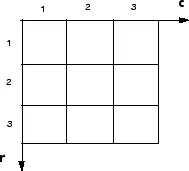
First part: If you are referring to the sign of curvature, you should notice the coordinate systems in an image or in a matrix and that of a plot. When we plot, as in your plot, usually the lower-left corner corresponds to the minimum of both x- and y-axis. Whereas in an image coordinate system, you have something like:

The coordination (with row and column index) starts from the upper-left corner.

The other visual difference between the two curves is their absolute curvature, and that is due to nothing but the axis limits. If you set the axis limits to be equal you will see two equally bent curves. Use xlim and ylim for this purpose.


Second part: If you want to quantify the load / pressure / weight applied to the system, the absolute value of the coefficient of x^2 is a monotonic variable. Therefore you can rely on it solely and calibrate it with applying different known amounts of stress to the system.

Community
  • 1
  • 1
Erfan
  • 1,897
  • 13
  • 23
  • I am new to Matlab, how can I set axis limits? I like to get sure they are equal. What is the role of *mu*. Anyway, you didn't say how to quantify the degree of bending. – Ahmad Oct 13 '16 at 13:18
  • use [`xlim`](http://www.mathworks.com/help/matlab/ref/xlim.html) and [`ylim`](http://www.mathworks.com/help/matlab/ref/ylim.html) to set axis limits. To know all about [`polyval`](http://www.mathworks.com/help/matlab/ref/polyval.html) and its input arguments just check it out. – Erfan Oct 13 '16 at 13:26
1

Radius of curvature is (1 + (dy/dx)^2)^3/2 all over d^2y/dx^2.

Or to put it into pseudo code

     /*
         curvature of ax*x + b*x + c, given x
     */
     curvaturequad(a, b, c, x)
     {
        dybydx = 2*a*x + b;  // first derivative
        d2ybydx2 = 2 * a;    // second derivative

        dybydx2 = dybydx*dybybx;
        numerator = sqrt(dybydx2 + 1)*(dybydx +1);
        return numerator / d2ybydx2;
     }
Malcolm McLean
  • 6,258
  • 1
  • 17
  • 18
  • What's this? It's not MATLAB code (if it's pseudocode - please say so - so as not to confuse potential readers). Also it doesn't address the 1st part of the OPs question. – Dev-iL Oct 13 '16 at 13:11