This solution uses a Python implementation of this approach. The idea is to convolve the image with a special kernel that identifies starting/ending points in a line. These are the steps:
- Resize your image a little bit, because its too big.
- Convert the image to grayscale
- Get the skeleton
- Convolve the skeleton with the endpoint kernel
- Get the coordinates of the endpoints
Now, that would be first iteration of the proposed algorithm. However, depending on the input image, there could be duplicated endpoints - individual points that are too close to each other and could be joined. So, let's incorporate some additional processing to get rid of such duplicated points.
- Identify possible duplicated points
- Join the duplicated points
- Compute final points
These last steps are too general, let me further elaborate on the idea behind the duplicates elimination when we get to that step. Let's see the code for the first part:
# imports:
import cv2
import numpy as np

# image path
path = "D://opencvImages//"
fileName = "hJVBX.jpg"

# Reading an image in default mode:
inputImage = cv2.imread(path + fileName)

# Resize image:
scalePercent = 50  # percent of original size
width = int(inputImage.shape[1] * scalePercent / 100)
height = int(inputImage.shape[0] * scalePercent / 100)

# New dimensions:
dim = (width, height)

# resize image
resizedImage = cv2.resize(inputImage, dim, interpolation=cv2.INTER_AREA)

# Color conversion
grayscaleImage = cv2.cvtColor(resizedImage, cv2.COLOR_BGR2GRAY)
grayscaleImage = 255 - grayscaleImage
So far I've resized the image (to a 0.5 of the original scale) and converted it to grayscale (in reality an inverted binary image). Now, the first step to detect endpoints is to normalize the lines width to 1 pixel. This is achieved by computing the skeleton, which can be implemented using OpenCV's Extended Image Processing module:
# Compute the skeleton:
skeleton = cv2.ximgproc.thinning(grayscaleImage, None, 1)
This is the skeleton:

Now, let's run the endpoint detection portion:
# Threshold the image so that white pixels get a value of 0 and
# black pixels a value of 10:
_, binaryImage = cv2.threshold(skeleton, 128, 10, cv2.THRESH_BINARY)

# Set the end-points kernel:
h = np.array([[1, 1, 1],
              [1, 10, 1],
              [1, 1, 1]])

# Convolve the image with the kernel:
imgFiltered = cv2.filter2D(binaryImage, -1, h)

# Extract only the end-points pixels, those with
# an intensity value of 110:
endPointsMask = np.where(imgFiltered == 110, 255, 0)

# The above operation converted the image to 32-bit float,
# convert back to 8-bit uint
endPointsMask = endPointsMask.astype(np.uint8)
Check out the original link for information on this method, but the general gist is that the kernel is such that convolution with ending points in a line will produce values of 110, as a result of neighborhood summation. There are float operations involved, so gotta be careful with data types and conversions. The result of the procedure can be observed here:

Those are the endpoints, however, note that some points could be joined, IF they are too close. Now comes the duplicate elimination steps. Let's first define the criteria to check if a point is a duplicate or not. If the points are too close, we will join them. Let's propose a morphology-based approach to points closeness. I'll dilate the endpoints mask with a rectangular kernel of size 3 and 3 iterations. If two or more points are too close, their dilation will produce a big, unique, blob:
# RGB copy of this:
rgbMask = endPointsMask.copy()
rgbMask = cv2.cvtColor(rgbMask, cv2.COLOR_GRAY2BGR)

# Create a copy of the mask for points processing:
groupsMask = endPointsMask.copy()

# Set kernel (structuring element) size:
kernelSize = 3
# Set operation iterations:
opIterations = 3
# Get the structuring element:
maxKernel = cv2.getStructuringElement(cv2.MORPH_RECT, (kernelSize, kernelSize))
# Perform dilate:
groupsMask = cv2.morphologyEx(groupsMask, cv2.MORPH_DILATE, maxKernel, None, None, opIterations, cv2.BORDER_REFLECT101)
This is the result of the dilation. I refer to this image as the groupsMask:

Note how some of the points now share adjacency. I will use this mask as a guide to produce the final centroids. The algorithm is like this: Loop through the endPointsMask, for every point, produce a label. Using a dictionary, store the label and all centroids sharing that label - use the groupsMask for propagating the label between different points via flood-filling. Inside the dictionary we will store the centroid cluster label, the accumulation of the centroids sum and the count of how many centroids where accumulated, so we can produce a final average. Like this:
# Set the centroids Dictionary:
centroidsDictionary = {}

# Get centroids on the end points mask:
totalComponents, output, stats, centroids = cv2.connectedComponentsWithStats(endPointsMask, connectivity=8)

# Count the blob labels with this:
labelCounter = 1

# Loop through the centroids, skipping the background (0):
for c in range(1, len(centroids), 1):

    # Get the current centroids:
    cx = int(centroids[c][0])
    cy = int(centroids[c][1])

    # Get the pixel value on the groups mask:
    pixelValue = groupsMask[cy, cx]

    # If new value (255) there's no entry in the dictionary
    # Process a new key and value:
    if pixelValue == 255:

        # New key and values-> Centroid and Point Count:
        centroidsDictionary[labelCounter] = (cx, cy, 1)

        # Flood fill at centroid:
        cv2.floodFill(groupsMask, mask=None, seedPoint=(cx, cy), newVal=labelCounter)
        labelCounter += 1

    # Else, the label already exists and we must accumulate the
    # centroid and its count:
    else:

        # Get Value:
        (accumCx, accumCy, blobCount) = centroidsDictionary[pixelValue]

        # Accumulate value:
        accumCx = accumCx + cx
        accumCy = accumCy + cy
        blobCount += 1

        # Update dictionary entry:
        centroidsDictionary[pixelValue] = (accumCx, accumCy, blobCount)
Here are some animations of the procedure, first, the centroids being processed one by one. We are trying to join those points that seem to close to each other:

The groups mask being flood-filled with new labels. The points that share a label are added together to produce a final average point. It is a little hard to see, because my label starts at 1, but you can barely see the labels being populated:

Now, what remains is to produce the final points. Loop through the dictionary and check out the centroids and their count. If the count is greater than 1, the centroid represents an accumulation and must be diveded by its count to produce the final point:
# Loop trough the dictionary and get the final centroid values:
for k in centroidsDictionary:
    # Get the value of the current key:
    (cx, cy, count) = centroidsDictionary[k]
    # Process combined points:
    if count != 1:
        cx = int(cx/count)
        cy = int(cy/count)
    # Draw circle at the centroid
    cv2.circle(resizedImage, (cx, cy), 5, (0, 0, 255), -1)

cv2.imshow("Final Centroids", resizedImage)
cv2.waitKey(0)
This is the final image, showing the end/starting points of the lines:
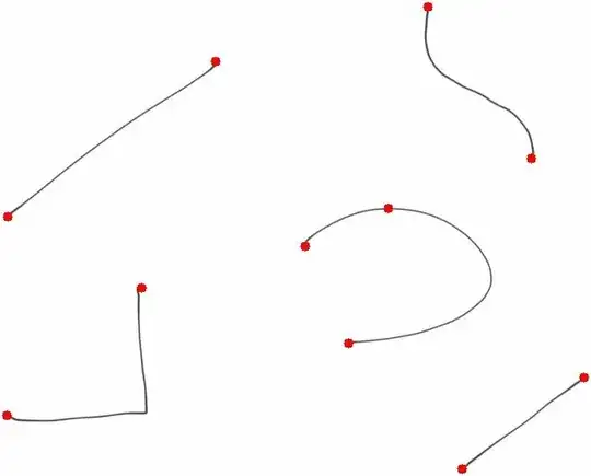
Now, the endpoints detection method, or rather, the convolution step, is producing an apparent extra point on the curve, that could be because of a segment on the lines is too separated from its neighborhood - splitting the curve in two parts. Maybe applying a little bit of morphology before the convolution could get rid of the problem.


